- Mohammed K and Srichitra S
- June 3, 2024
VSLAM Series – Feature Extraction & Description Pipeline
Introduction
This Series of blogs explores the exciting field of Feature based Visual Simultaneous Localization and Mapping (VSLAM). It also discusses the two state-of-the-art algorithms that are widely used in this area: RTAB-Map and ORB-SLAM3. After going through our earlier blog on the challenges of SLAM and the advantages of using cameras for SLAM, this new article provides a comprehensive study of different components of feature based visual SLAM algorithms, including their underlying principles. The blog provides a comparison of the two algorithms, discussing their strengths and weaknesses and identifies the best use cases for each algorithm.
SLAM utilizes different types of sensors, including LiDARs, cameras, and radar, to estimate the robot’s location and map the surrounding environment. However, each method has its strengths and limitations, and the use of multiple sensors is often required to improve accuracy and reduce errors. The cameras are a popular sensor for visual SLAM (VSLAM), which addresses the challenge of accurately localizing and mapping a robot’s surroundings using visual information. VSLAM is increasingly popular due to low-cost sensors, easy sensor fusion, and GPS-denied operation, making it practical for autonomous navigation. The first part of the blog will explore the key concepts and techniques of feature extraction and description pipeline of VSLAM.
Common Modules for a Feature-based Visual Slam
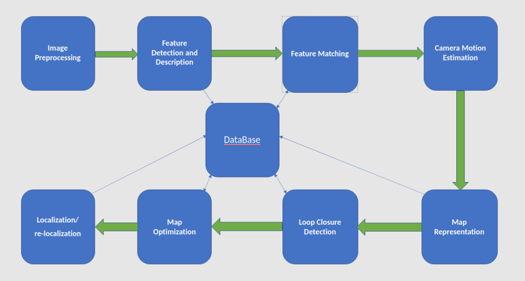
A feature-based visual SLAM system typically consists of several modules that work together to estimate the camera pose and build a map of the environment. Figure 1 shows the common modules of a feature-based visual SLAM system.
-
- Image Preprocessing: This module performs image preprocessing operations such as undistortion, color correction, and noise reduction to prepare the images for feature extraction.
- Feature Detection and Description: This module extracts distinctive features from the images and describes them using a set of descriptors. Common feature detection algorithms include FAST, ORB, and SURF, while common descriptors include SIFT, ORB, and FREAK.
- Feature Matching: This module matches the features between consecutive images or between distant images using a matching algorithm such as brute-force matching, FLANN, or ANN. The matches are used to estimate the camera motion and to build a map of the environment.
- Camera Motion Estimation: This module estimates the camera motion from the matched features using techniques such as direct sparse odometry (DSO), visual-inertial odometry (VIO), or simultaneous localization and mapping (SLAM).
- Map Representation: This module represents the map of the environment using a data structure such as a point cloud, a keyframe graph, or a pose graph. The map is updated and optimized continuously as new images and features are added.
- Loop Closure Detection: This module detects loop closures, which occur when the camera revisits a previously visited location and helps to reduce the drift in the camera motion estimation. Loop closure detection is typically performed using techniques such as bag-of-words (BoW) or covisibility graph.
- Map Optimization: This module optimizes the map and the camera poses using techniques such as bundle adjustment, pose graph optimization, or SLAM back-end. Map optimization helps to refine the accuracy and consistency of the map and to reduce the error in the camera motion estimation.
- Localization and re-localization: This module performs localization and re-localization, which is the task of estimating the camera pose in a known and unknown map. Localization is typically performed using techniques such as particle filtering, Monte Carlo localization, or pose-graph optimization.
The choice of modules and algorithms depends on the specific requirements of the application, such as the type of sensor, the computational resources, the accuracy, and the robustness.
Feature Detection and Description
The first step of feature-based visual SLAM (Simultaneous Localization and Mapping) is to extract features from the images captured by the camera. To make it more computationally efficient, the image is first converted into a grayscale image before the feature extraction step. Any specific, identifiable or characteristic part of an image that can be used to distinguish it from other images is called a feature. It could be as simple as edges and corners or even complex like shapes, textures or patterns that change in viewpoint, illumination and scale.
Feature extraction is performed using a feature detection algorithm, such as the Harris corner detector, Scale-Invariant Feature Transform (SIFT), Speeded-Up Robust Feature (SURF), or Oriented FAST and Rotated BRIEF (ORB). ORB is a popular choice for feature detection and extraction due to its efficiency, robustness, and rotation invariance. It uses a combination of FAST keypoint detection and BRIEF binary descriptor to accurately detect and describe features in images. ORB is computationally efficient, operates in real-time on low-power devices, and is robust to noise, blur, and low contrast or lighting conditions. It is useful in applications such as outdoor navigation and surveillance.
The ORB algorithm uses an image pyramid to detect features at different scales in an image. The pyramid is created by down sampling the original image to create a series of smaller images, with each level having a lower resolution than the previous level. By detecting features at multiple scales, the algorithm becomes more robust to changes in image scale, and the pyramid also helps to reduce computational complexity.
Feature Detection Algorithms
FAST (Features from Accelerated Segment Test)
After the creation of the image pyramid, the ORB algorithm performs Feature Detection by using the FAST (Features from Accelerated Segment Test) algorithm to detect key points in each level of the image pyramid. The FAST algorithm can be defined as follows:
1. Choose a pixel p in the image and a threshold value t.
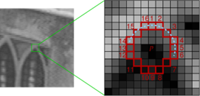
2. Select a circular ring around the pixel p with radius r and choose a set of n pixels on the ring.
3. Compute the difference between the intensity of pixel p and the intensity of each of the n pixels on the ring.
4. If at least k pixels out of the n have intensities greater than p + t or less than p – t, then pixel p is considered a corner or a keypoint.
The above process is repeated for all pixels in the image.
The FAST algorithm is efficient because it only requires a small number of intensity comparisons to determine if a pixel is a corner or keypoint. This makes it well-suited for real-time applications. Then a non-maximum suppression is to be applied to eliminate redundant feature points in close proximity. The process of non-maximum suppression can be broken down into two steps:
Step 1: Compute score function (S) for all the detected feature points. The score function is typically computed as the sum of the absolute difference between the central pixel P and the values of its surrounding n pixels.

Step 2: If two adjacent feature points have overlapping regions, the one with the lower S value is discarded or suppressed. This step ensures that only the highest-scoring feature points are retained (see figure 3).

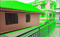
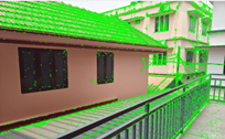
After feature detection the ORB uses centroid orientation to compute the dominant orientation of feature points based on local gradients for rotation invariance. to compute the intensity centroid of a patch of pixels around a keypoint, ORB follow the steps outlined below:
1. Compute the horizontal and vertical gradients of the patch using the Sobel operator: Let’s assume that we have a patch of pixels P of size n x n centered around the keypoint. The horizontal gradient Gx(i,j) and vertical gradient Gy(i’j) at pixel (i,j) in the patch are given by:


The gradient vector G(i,j) at pixel (i,j) is given by: G (i,j)=[Gx (i,j),Gy (i.j)]
2. The distance d(i,j) of pixel (i,j) from the center of the patch is given by:

The product of the gradient vector and the distance is given by:
W (i,j)= G (i,j)*d (i,j), where * denotes the element-wise multiplication of two vectors.
Then sum the values of W(i,j) over all pixels (i,j) in the patch to get the weighted sum:
![]() over all pixels (i,j) in the patch.
over all pixels (i,j) in the patch.
where i and j denote the row and column indices of the pixel in the patch, and P(i,j) is the intensity value of the pixel
3. Compute the sum of magnitudes of gradient of all pixels in the patch as:
![]() over all pixels (i,j) in the patch.
over all pixels (i,j) in the patch.
4. Compute the intensity centroid (cx, cy) of the patch as:


, where (n+1)/2 represents the center of the patch.
5. Compute the orientation: the orientation of the keypoint is calculated by taking the angle between the intensity centroid and the keypoint. This is given by:

where arctangent function that takes the signs of the numerator and denominator into account to return an angle between ![]() and
and ![]() .The orientation computed in the above is assigned to the keypoint as its dominant orientation. If there are multiple orientations that are significantly high, then additional keypoints are created for each of these orientations.
.The orientation computed in the above is assigned to the keypoint as its dominant orientation. If there are multiple orientations that are significantly high, then additional keypoints are created for each of these orientations.
BRIEF (Binary robust independent elementary feature)
BRIEF is a binary descriptor that can be calculated from FAST keypoints. The key points are described by comparing their surrounding pixel values in a predefined pattern. Brief uses a randomized set of pairs of pixels, compares their intensities, and assigns a binary value to each pair based on the comparison result. The binary values from all the pairs are concatenated into a single binary string, which forms the feature descriptor for the key point. The length of the binary string is typically fixed, and the number of pairs used in the comparison is also limited. The resulting binary feature vector is therefore relatively small in size, making it computationally efficient to use in large-scale image processing applications.
Brief start by smoothing image using a Gaussian kernel of size (7, 7) in order to prevent the descriptor from being sensitive to high-frequency noise. Then a patch is defined as a square region of the image centered around a keypoint location. The size of the patch is typically chosen to be a fixed number of pixels in width and height. Then BRIEF selects a random pair of pixels in a defined patch around the keypoint and creates a 2 x n Matrix M.

Using the patch orientation and the corresponding rotation matrix, we construct a “rotated” version ![]() of M.
of M. ![]()
Now, the rotated BRIEF operator becomes: ![]()
The feature is defined as a vector of n binary tests: ![]() , where
, where ![]() is defined as:
is defined as: ![]()
Finally, the method computes the BRIEF descriptor for the keypoint using the selected set of pixel pairs from ![]()
Bag of visual words (BoVW)
BoVW uses the concept of visual words, which are similar to the words in natural language. Each visual word represents a cluster of similar features, such as SIFT or ORB descriptors, that occur frequently in the images.
The process of computation of BoVW is as follows: 
- Let X be the set of images in the dataset, and let F(x) be the set of local features extracted from image x. Let K be the number of visual words and let
 be the set of visual words obtained by clustering the features in F(x). Given a set of N feature points x1, x2, …, xN in d-dimensional space, the K-means algorithm partitions the feature points into K clusters
  . Each cluster is represented by its centroid or mean, denoted by the vector. At each iteration of the algorithm, we minimize the within-cluster sum of squared distances (WCSS), defined as:
- Where xi is a data point and uk is the centroid of the cluster to which xi is assigned. the centroid uk is the mean of the data points assigned to cluster k:
 for xi in Ck, where Ck is the number of data points assigned to cluster k.
 - Once the visual words are obtained, a histogram is generated for each image in the dataset. The histogram counts the occurrences of each visual word in the image. Specifically, for each image, we count the number of features assigned to each visual word and store the counts in a histogram. This results in a fixed-length vector representation of each image, where the dimensions correspond to the visual words and the values correspond to the counts of each visual word in the image. For each image x in X, we compute its histogram H(x), where is the number of features in F(x) that are assigned to visual word. The final step is to normalize the histogram vectors to make them invariant to changes in the image scale and illumination. This is done by applying L2 normalization to each histogram vector, which scales the vector to have unit length. The L2 normalization is computed as follows:
 for i = 1 to K
By comparing the histograms of visual words between successive images, the method can estimate the camera’s motion and the locations of the keypoints in 3D space.
Conclusion
The feature extraction pipeline is a critical component of visual SLAM systems, as it enables the extraction of distinctive and robust visual features from sensor data. The pipeline typically involves a series of steps such as image acquisition, pre-processing, feature detection and feature description. The quality and efficiency of the pipeline directly affect the accuracy and robustness of the SLAM system, as well as its ability to operate in real-time.
To design an effective feature extraction pipeline for visual SLAM, it is important to carefully select and optimize each step of the pipeline based on the specific requirements of the application. This includes selecting appropriate feature detection and description algorithms, optimizing feature matching strategies, and addressing potential issues such as occlusion, dynamic scenes, and lighting variations.
In conclusion, a well-designed and optimized feature extraction pipeline is essential for the success of visual SLAM systems, as it directly influences accuracy, robustness, and real-time performance. By carefully selecting and tuning each step of the pipeline to address specific application requirements and challenges, visual SLAM can achieve reliable and efficient localization and mapping in a wide range of scenarios.

