High-speed nut counting based on Computer Vision

“I feel the need, the need for speed”, a famous quote from the Hollywood movie ‘Top Gun’ rings true for most engineers. We strive to make existing algorithms, software and hardware run faster and faster. This blog post explains the design of one such high-speed, high-accuracy solution developed by Ignitarium engineers: a computer vision based solution for industrial part counting. Such automated industrial solutions are increasingly seeing demand in factories across the world, as they struggle to cut down labor costs and increase productivity of their assembly lines. 

Ignitarium worked with a class-leading image sensor company to demonstrate the capabilities of their 90 FPS high resolution sensor in an industrial use case for part counting, specifically nut counting.

Calculations:

• Camera capture speed – 90 FPS. 90 frames per second translates to 11ms. So, all the operations ranging from image capture to display that had to be set up for nut counting were to be executed in just 11ms. If total end to end system latency exceeds 11ms, then we lose the frames because the camera is always going to write new frames at this speed.

Problem statement for building the nut counting solution

To demonstrate this image sensor’s performance at 90FPS, fast moving objects had to be used. The camera can then capture images of these fast moving objects and software can process those images. Simulating such high speeds was made possible by building a rotating system instead of a linear one. 

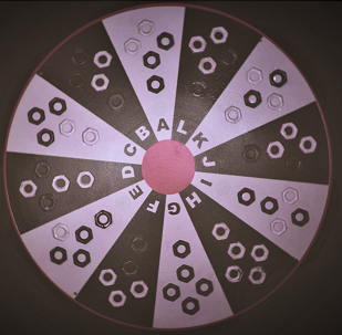
A high-speed rotating platform was created as shown in Fig. 1. It had 12 sectors, named alphabetically from A to L. Each sector has multiple slots into which a variable number of nuts can be inserted by the user. When the disk starts rotating, the camera captures the images, the algorithm counts the nuts in each sector and the final count is displayed on the screen. Sounds simple? It’s not so in reality. 

Challenges faced 

Interface constraints

Since the camera’s image capture pipeline was still under development, it was decided to use an FPGA based board as the development platform. Due to limited support for today’s trending Deep Learning frameworks (read : TF, Keras, Torch) on the specific platform, it was decided to adopt a software-only approach for all components in the pipeline post image capture. In other words, compute and display was handled purely in software running on a standard embedded processor rather than hardware accelerators. Specifically, we chose a classical image processing approach to keep the compute requirements light.

The pipeline consisted of cropping the segment first. Then deciding the dominant color of the sector. Then comes the contour finding and ultimately counting only the nuts. Finally, the nut count is displayed alongside the sector name. 

Software issues

Memory copy

The device had a sensor pipeline which would dump frames continuously into the shared DDR memory. Shared memory has a physical address. And since we were using components like openCV for image processing and basic display functionality for output, we required an OS. Chosen OS was petalinux. There were many instances where python was making a copy of the data. This copy time itself was exceeding the acceptable pipeline latency. To solve this, each and every line of the code was reviewed and rewritten in some cases. To avoid copy of the memory, memory mapping functionality was used to map the physical address of shared memory to virtual address.

OpenCV libraries

OpenCV’s resize function can spring a few surprises while working on low level code. Experienced users can understand the basic syntax like output_image=resize(input_image, dimensions). In this situation, an inherent copy of the input_image was getting created.. To solve this issue, we wrote our custom image resizing function based on sampling.It was a lossy method, but worked perfectly for the given application.

System level issues

Position calibration

In order to detect a sector properly, the user needs to place the rotating disk precisely under the camera such that the camera’s principal axis (an imaginary line going through the center of lens) should coincide with the centre of the red circle shown Fig. 1. This proved to be a practical challenge. We found human error in a) wrong vertical displacement and b) disk going out of the frame.

In order to tackle this problem, we created a calibration mechanism. By taking reference to the central red circle, the calibration algorithm was designed to handle errors in the mounting position. Vertical mounting errors were avoided by measuring the pixel area of the central circle and limiting it within an acceptable range. Misaligned position errors were reported by taking reference to an imaginary rectangle within an image. The auto-detected positions would be overlaid with colored markers via a user-friendly UI on a display allowing the calibration loop to be closed. 

Lighting

AI-enabled algorithms can handle changes in brightness well. But classical image processing methods used here lack that level of robustness. Of course, it is possible to implement global methods like histogram equalization etc., on each frame, but again, that would add to the processing time.

There is a huge difference in the images captured during a well-lit environment during day vs dimly lit environment during night. Moreover, artificial lighting doesn’t help much because it is a high speed image capture. One needs more and more lighting for higher frame rate capture.

We tackled this problem by lighting-based calibration. The central red circle was analysed in different light conditions and favourable ranges of it’s HSV values were calibrated. In case the surrounding lighting is dimmer or brighter than the expected range, an error display mechanism was added to the system. By looking at the error on the terminal, the user can dial up or down the lighting controls built into the rotary system, to the suitable setting.

Conclusion

In conclusion, I wanted to share some learnings with all the image processing, computer vision and deep learning practitioners. As engineers, we develop and experiment in the sandbox environment many times. Good compute resources are available most of the time without any latency constraints. Playing around with a real life system is really interesting and imparts immense learning. The challenges are real and one needs to think at a basic level to address them. In this case of building a nut counting solution, we deployed linux basics, C, python, openCV, embedded, image processing, computer vision and camera calibration skills on just a single project.