1. Introduction
Before we dive in to Homography, let’s understand image stitching with the help of the block diagram in Figure 1.
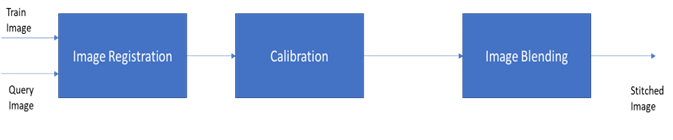
The input to image stitching is a pair of images which are treated as Train image and Query image. These two images will undergo a Registration process, which involves identifying features from the individual images. This process of image registration uses popular techniques like SIFT, ORB etc., which have been embedded in OpenCV libraries. The extracted features are then fed to the next block, called the Calibration block, which will match the features between the two and come up with a model to estimate the translation/rotation between the two images. The Brute force method or K-means can be used to find closest matches and then fed to RANSAC (Random Sample Consensus) to learn and predict the model. This is where the Homography matrix comes in, dictating the match between the two images in terms of a parametric model. The third stage, Image Blending, is the process which involves transformation of one of the images by using homography matrix as warp perspective and then aligning with another image to blend as a single high-resolution image.
2. 2D transformations
Let’s first understand the 2D transformation types that our images are generally subjected to.
2.1 Translation
2D translation can be picturized in matrix form as below:
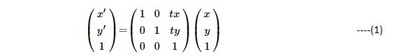
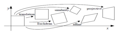
As you can see, pixels at (x,y) locations are transformed to x’(x’ = x + tx ) and y’(y’= y + ty). From Figure 2, the rectangular box marked as ‘translation’ is shifted to new locations of (x’,y’). The above matrix representation is generic to represent any 2D-transformation. The 3rd row of the matrix is just for ensuring that we have a full rank of 3×3 matrix.
Now, let’s start adding more variabilities to the matrix to enable different transformations.
2.2 Rotation + Translation
Adding rotation to transformation of Equation (1), leads us to:
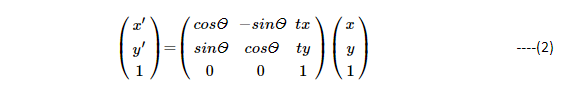
Where Ѳ is the amount of pixel rotation. Here in Equation (2), we can represent rotation matrix as:
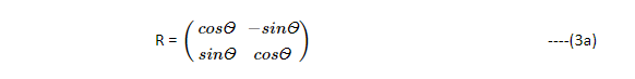
R is an orthonormal rotation matrix, satisfying RRᵀ = I and ‖R‖=1.
(Where ᵀ represents the transpose operation)
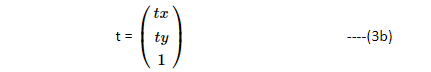
The Translation vector is,
Equation (2) can be written in the linear system of equations as:
X’ = RX + T
where X’ = (x’, y’, 1)ᵀ , the new pixel coordinates
original pixel coordinates X = (x,y,1)ᵀ
Rotation, R as in equation (3a)
Translation T=(tx,ty,1)ᵀ)
2.3 Affine
The affine transformation can be represented as:
The affine is an indication that transformation is such that parallel lines remain parallel (which inherits the property of affine where a+b =1), hence yielding affine transformation. Consider a rectangular box positioned such that its origin is where (x,y) = (0,0). Observe that in Figure 2, the lines (edges) of the rectangular box, remained parallel post affine transformation.
A few important properties worth noting here are :
- Origin of the box does not necessarily map to the origin after transformation.
- Lines map to lines
- Parallel lines remain parallel
- Closed solution under composition. (Under this transformation, the transformation parameters can be found with unique parameters)
2.4 Projective
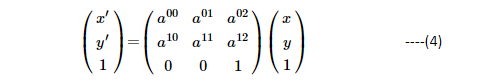
The projective transformation is also known as perspective transform or homography. This transformation operates on homogenous coordinates as:

Where H is 3×3 matrix embedding the 8 degrees of freedom.
Here the transformations are as follows:
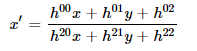
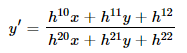
This generates a Homography matrix of the form:
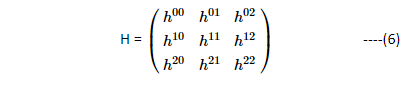
Where h22 is normalized to a value of 1. As you can visualize here, the Homography transformations give 8 degrees of freedom from h00toh21. These can be correlated to Rotation (R), translation (t) (refer equation (3a and 3b)) and scaling (S).
Consider a rectangular box positioned at the origin where (x,y) = (0,0) as in Figure 2. After transformation, the box can be seen transformed to the extreme right.
A few important properties worth noting here are:
- Origin of the box does not necessarily map to origin
- Lines map to lines
- Parallel lines do not necessarily remain parallel
- Closed solution under composition
As you can see difference between Affine and homography / projective transformations is that parallel lines won’t remain parallel due to the additional 2 degrees of freedom that was brought in the form of h20 and h21, which indicates z direction of rotations.
Table 1 summarizes the transformations:
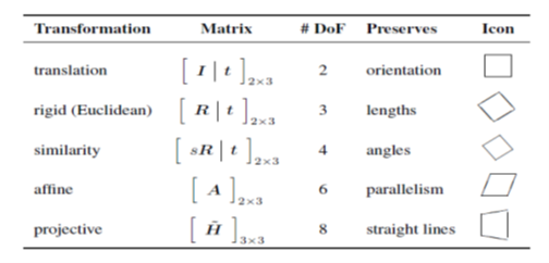
These properties are useful when we are transforming one image to another image, where they have limited overlap between them, and the camera rotations or variations are embedded with 8 degrees of freedom. You can interpret Homography matrix as rotation along x,y,z direction and translation along x and y directions, keeping z-direction translation constant to 1, and adhering to the following:

3. Perspective projection
The following is required to create the parametric model of camera acquisition. In Figure 3., F represents the train image frame (current or reference frame) and F* represents the query image (desired frame, as we want to align to the desired one and stitch). The camera observes a planar object, consisting of a set of n 3D feature points, P, with cartesian coordinates
P =(X,Y,Z)
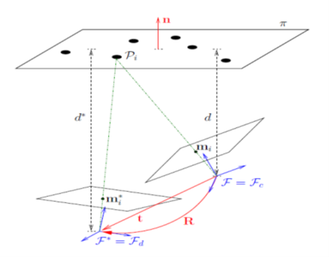
The d and d* represent respective distances from object plane to corresponding camera frame. The normal ‘n’ to the plane can be referred to the reference or current frame. The camera grabs an image of the object from both desired (query) and current (reference) settings, which implies 3D points on a plane so that they have the same depth from corresponding camera origin. The homogenous transformation matrix, converting 3D point coordinates from the desired frame to the current frame is
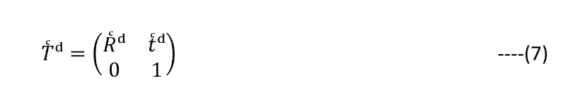
Here R and t are the rotation matrix and translation vector respectively. This allows Euclidian reconstruction from homography as follows:

Notice that n, normalized vector, is embedded, which ensures normality to object plane.
The above equation also indicates that there is possibility of extraction of individual components R, t and n.
3.1 Singular Value Decomposition (SVD):
The closed form solutions are obtained numerically with the help of SVD decomposition. {Ref. [1]}.
The eigen values and eigen vectors give a picture of which vector/value undergoes variations.
Hence,

Where Λ={λ₁ ,λ₂, λᴣ} , Eigen Values in descending order
V = [v₁,v₂,vᴣ] , corresponding Eigen Vectors
The eigen values can also be obtained directly from H using Equation (5) using
HX = λX’ , where λ are the eigen values.
The eigen values obtained using the above formula (H-λI) = 0 (Where I is an identity Matrix), may give complex eigen values, which are difficult to analyze. Hence SVD decomposition of Equation (9) nicely gives diagonal elements which are square of eigen values. The square root gives eigen values, which can be interpreted, and important properties can be derived as follows:
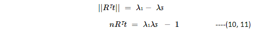
As in Equation (8), the Homography contains Rotation, translation, and normal vector. This defines translation vector, which is normalized as:
eigen vectors are,
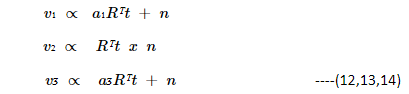
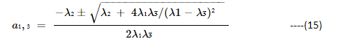
The a1, a3 are scalars , defined as
4. Properties helpful to align images
Consider 3 cases of study to understand how to utilize Homography properties of Equations (10 to 15). We use the following two sets of images to showcase the insights obtainable from Homography. The Train and Query images of Figures 4 and 5 are fed into the block diagram of Figure 1 and we get Homography matrix as per the cases below:
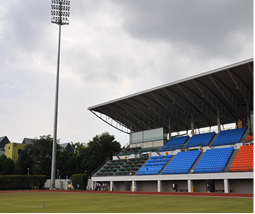
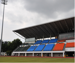
Figure 4: Desired (query) and current (train) frames
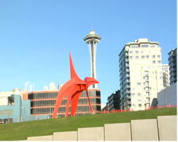
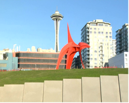
Figure 5: Desired (query) and current (train) frames
Case 1 : Train Image and Query Image are the same
When the left image from Figure 4 is fed in to Figure 1 both as train and query image, we get:
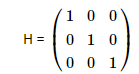
eigen values, λ=(1,1,1)
This means Equations (10,11) translate to
||Rᵀt|| = 0
nRᵀt = 0
What this means is that there is no translation between the two images. This conclusion helps when we encounter the same images either repeated or very similar (close to 100% overlap), we can find translation vector and normal to conclude that images are the same and hence no alignment is required. Additionally, the confidence on this derivation can be improved with the following parameters:
Inlier ratio: Number of features matched between two images / Total number of features between two images = 10228/10228 = 100 %
The determinant of H = 1, indicates volume is 1.
Also, eigen values are 1, indicating the variations are uniform and if we draw ellipse of the eigen values axis, we get a circle indicating that in any direction you take, there is uniform variation, which in turn indicates no translation.
Right: stitched image (scaled to fit to page)
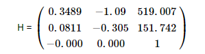
Case 2: Train and Query Images with some percentage of overlap, but images are different
The query and train images from Figure 4 are fed for stitching. Please note that train image has extra red seating of stadium and camera frame has moved closer to the flood lights, as compared to query image. There is some overlap seen in train image with respect to query image.
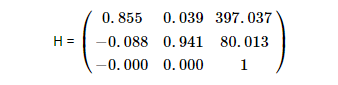
eigen values, λ=(405.0214,0.9499,0.00216)
This means translation is:
||Rᵀt||= 405.0214 – 0.00216 = 405.0192
nRᵀt = 405.0214*0.00216 – 1 = -0.125
Let us understand the meaning of these values from the ellipse drawn in Figure 7.
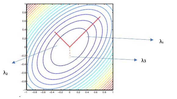
As you see above, the ellipse major axis is driven by λ₁, and smaller axis by λ₂, with normalized z-plane by λᴣ. As the rotation and translation together are significant, the major axis of ellipse dictates the Rᵀt , which is a major contributor for change in two images, hence variance along this axis is high. The second eigen value is close to 1, gives an indication along this axis, the features are common and hence there is no variation along this axis between the two images. Last eigen value is along z-direction which is close to zero, indicating that in the z-direction there is no change, hence nRᵀt ~ 0.
Thus,
λ1>> λ2=1>>λᴣ 𝝀𝟏>>𝝀𝟐=𝟏>>𝝀ᴣ
—(16)
is an indication that we have got some amount of rotation and translation. This property is very useful to know how much variation exists between two images.
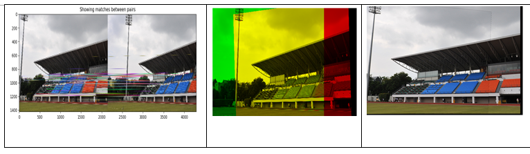
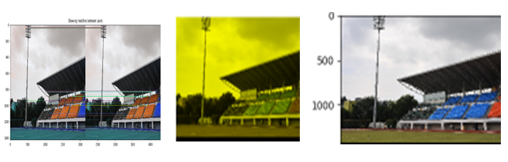
Right: stitched image (scaled to fit to page)
In the middle image, the yellow color shade indicates common features and green and red are respectively the new features from query and train images. As you can see the stitched image covers the extra red seating of the stadium.
The techniques described between Equations 10-15 are efficiently applied to get to the stitched image as above. Even while selecting RANSAC threshold, we utilized these properties to arrive at the threshold, to give optimal homography.
Another confidence builder to this is that we get inlier ratio of 4558/4990, which translates to 91.3% features are found to be common. The determinant of Homography is 0.833, which also indicates the matrix is nonsingular.
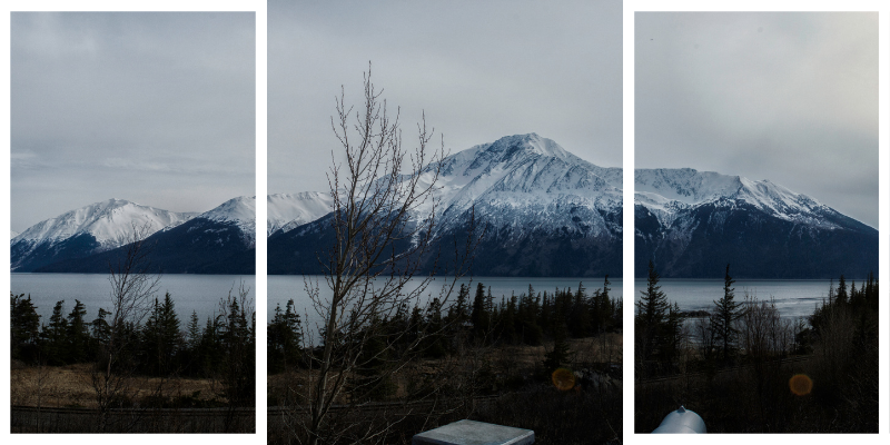
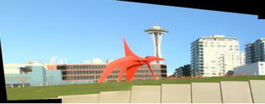
Another stitching established with help of above techniques for the images in Figure 5 are:
Case 3: Train and Query Images are different
Let’s feed left part of Figure 4 and left part of Figure 5, which are entirely different to see its effect. Let’s first see the Homography:
Determinant of H = 1.929×10⁻⁶ (~0), which clearly indicates it is a singular matrix. Hence the volume covered by determinant is close to zero, indicating no common features between the two images. So, no alignment exists between the two images.
Inlier ratio = 26/1658 = 1.5%, these features which have appeared as common are due to noise or image registration imperfections.
5. Conclusion
The paper introduces how to use homography for detecting alignment of images and hence helping in image stitching. Stitching results are discussed using 2 image sets. The properties derived using eigen values are giving more value in terms of translation and rotation effects. These properties can be effectively applied in infrastructure analytics use cases (eg. Wind Turbine blade stitching) where many a time, imperfectly stabilized cameras are mounted on drones or crawler robots.
References:
[1]: https://hal.inria.fr/inria-00174036/PDF/RR-6303.pdf
[2]: https://www.researchgate.net/publication/262261060_Determinant_of_homography-matrix-based_multiple-object_recognition
[3]: http://szeliski.org/Book/
[4]: Handbook of Mathematical Models in Computer Vision, pages 273–292, Springer, 2005